The problem with building a device that is good at keeping secrets is that it turns users into the weakest link.
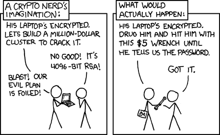
From xkcd, CC-BY-NC 2.5
In practice, attackers need not go nearly as far as rubber-hose cryptanalysis to obtain passwords; a simple inspection checkpoint, verbal threat or subpoena is often sufficiently coercive.
Most security schemes facilitate the coercive processes of an attacker because they disclose metadata about the secret data, such as the name and size of encrypted files. This allows specific and enforceable demands to be made: “Give us the passwords for these three encrypted files with names A, B and C, or else…”. In other words, security often focuses on protecting the confidentiality of data, but lacks deniability.
A scheme with deniability would make even the existence of secret files difficult to prove. This makes it difficult for an attacker to formulate a coherent demand: “There’s no evidence of undisclosed data. Should we even bother to make threats?” A lack of evidence makes it more difficult to make specific and enforceable demands.
Thus, assuming the ultimate goal of security is to protect the safety of users as human beings, and not just their files, enhanced security should come hand-in-hand with enhanced plausible deniability (PD). PD arms users with a set of tools they can use to navigate the social landscape of security, by making it difficult to enumerate all the secrets potentially contained within a device, even with deep forensic analysis.
Precursor is a device we designed to keep secrets, such as passwords, wallets, authentication tokens, contacts and text messages. We also want it to offer plausible deniability in the face of an attacker that has unlimited access to a physical device, including its root keys, and a set of “broadly known to exist” passwords, such as the screen unlock password and the update signing password. We further assume that an attacker can take a full, low-level snapshot of the entire contents of the FLASH memory, including memory marked as reserved or erased. Finally, we assume that a device, in the worst case, may be subject to repeated, intrusive inspections of this nature.
We created the PDDB (Plausibly Deniable DataBase) to address this threat scenario. The PDDB aims to offer users a real option to plausibly deny the existence of secret data on a Precursor device. This option is strongest in the case of a single inspection. If a device is expected to withstand repeated inspections by the same attacker, then the user has to make a choice between performance and deniability. A “small” set of secrets (relative to the entire disk size, on Precursor that would be 8MiB out of 100MiB total size) can be deniable without a performance impact, but if larger (e.g. 80MiB out of 100MiB total size) sets of secrets must be kept, then archived data needs to be turned over frequently, to foil ciphertext comparison attacks between disk imaging events.
The API Problem
“Never roll your own crypto”, and “never roll your own filesystem”: two timeless pieces of advice worth heeding. Yet, the PDDB is both a bit of new crypto, and a lot of new filesystem (and I’m not particularly qualified to write either). So, why take on the endeavor, especially when deniability is not a new concept?
For example, one can fill a disk with random data, and then use a Veracrypt hidden volume, or LUKS with detached partition headers. So long as the entire disk is pre-filled with random data, it is difficult for an attacker to prove the existence of a hidden volume with these pre-existing technologies.
Volume-based schemes like these suffer from what I call the “API Problem”. While the volume itself may be deniable, it requires application programs to be PD-aware to avoid accidental disclosures. For example, they must be specifically coded to split user data into multiple secret volumes, and to not throw errors when the secret volumes are taken off-line. This substantially increases the risk of unintentional leakage; for example, an application that is PD-naive could very reasonably throw an error message informing the user (and thus potentially an attacker) of a supposedly non-existent volume that was taken off-line. In other words, having the filesystem itself disappear is not enough; all the user-level applications should be coded in a PD-aware fashion.
On the other hand, application developers are typically not experts in cryptography or security, and they might reasonably expect the OS to handle tricky things like PD. Thus, in order to reduce the burden on application developers, the PDDB is structured not as a traditional filesystem, but as a single database of dictionaries containing many key-value pairs.
Secrets are overlaid or removed from the database transparently, through a mechanism called “Bases” (the plural of a single “Basis”, similar to the concept of a vector basis from linear algebra). The application-facing view of data is computed as the union of the key/value pairs within the currently unlocked secret Bases. In the case that the same key exists within dictionaries with the same name in more than one Basis, by default the most recently unlocked key/value pairs take precedence over the oldest. By offering multiple views of the same dataset based on the currently unlocked set of secrets, application developers don’t have to do anything special to leverage the PD aspects of the PDDB.
The role of a Basis in PD is perhaps best demonstrated through a thought experiment centered around the implementation of a chat application. In Precursor, the oldest (first to be unlocked) Basis is always the “System” Basis, which is unlocked on boot by the user unlock password. Now let’s say the chat application has a “contact book”. Let’s suppose the contact book is implemented as a dictionary called “chat.contacts”, and it exists in the (default) System Basis. Now let’s suppose the user adds two contacts to their contact book, Alice and Bob. The contact information for both will be stored as key/value pairs within the “chat.contacts” dictionary, inside the System Basis.
Now, let’s say the user wants to add a new, secret contact for Trent. The user would first create a new Basis for Trent – let’s say it’s called “Trent’s Basis”. The chat application would store the new contact information in the same old dictionary called “chat.contacts”, but the PDDB writes the contact information to a key/value pair in a second copy of the “chat.contacts” dictionary within “Trent’s Basis”.
Once the chat with Trent is finished, the user can lock Trent’s Basis (it would also be best practice to refresh the chat application). This causes the key/value pair for Trent to disappear from the unionized view of “chat.contacts” – only Alice and Bob’s contacts remain. Significantly, the “chat.contacts” dictionary did not disappear – the application can continue to use the same dictionary, but future queries of the dictionary to generate a listing of available contacts will return only Alice and Bob’s key/value pairs; Trent’s key/value pair will remain hidden until Trent’s Basis is unlocked again.
Of course, nothing prevents a chat application from going out of its way to maintain a separate copy of the contact book, thus allowing it to leak the existence of Trent’s key/value pair after the secret Basis is closed. However, that is extra work on behalf of the application developer. The idea behind the PDDB is to make the lowest-effort method also the safest method. Keeping a local copy of the contacts directory takes effort, versus simply calling the dict_list() API on the PDDB to extract the contact list on the fly. However, the PDDB API also includes a provision for a callback, attached to every key, that can inform applications when a particular key has been subtracted from the current view of data due to a secret Basis being locked.
Contrast this to any implementation using e.g. a separate encrypted volume for PD. Every chat application author would have to include special-case code to check for the presence of the deniable volumes, and to unionize the contact book. Furthermore, the responsibility to not leak un-deniable references to deniable volumes inside the chat applications falls squarely on the shoulders of each and every application developer.
In short, by pushing the deniability problem up the filesystem stack to the application level, one greatly increases the chances of accidental disclosure of deniable data. Thus a key motivation for building the PDDB is to provide a set of abstractions that lower the effort for application developers to take advantage of PD, while reducing the surface of issues to audit for the potential leakage of deniable data.
Down the Rabbit Hole: The PDDB’s Internal Layout
Since we’re taking a clean-sheet look at building an encrypted, plausibly-deniable filesystem, I decided to start by completely abandoning any legacy notion of disks and volumes. In the case of the PDDB, the entire “disk” is memory-mapped into the virtual memory space of the processor, on 4k-page boundaries. Like the operating system Xous, the entire PDDB is coded to port seamlessly between both 32-bit and 64-bit architectures. Thus, on a 32-bit machine, the maximum size of the PDDB is limited to a couple GiB (since it has to share memory space with the OS), but on a 64-bit machine the maximum size is some millions of terabytes. While a couple GiB is small by today’s standards, it is ample for Precursor because our firmware blob-free, directly-managed, high write-lifetime FLASH memory device is only 128MiB in size.
Each Basis in the PDDB has its own private 64-bit memory space, which are multiplexed into physical memory through the page table. It is conceptually similar to the page table used to manage the main memory on the CPU: each physical page of storage maps to a page table entry by shifting its address to the right by 12 bits (the address width of a 4k page). Thus, Precursor’s roughly 100MiB of available FLASH memory maps to about 25,000 entries. These entries are stored sequentially at the beginning of the PDDB physical memory space.
Unlike a standard page table, each entry is 128 bits wide. An entry width of 128 bits allows each page table entry to be decrypted and encrypted independently with AES-256 (recall that even though the key size is 256 bits, the block size remains at 128 bits). 56 bits of the 128 bits in the page table entry are used to encode the corresponding virtual address of the entry, and the rest are used to store flags, a nonce and a checksum. When a Basis is unlocked, each of the 25,000 page table entries are scanned by decrypting them using the unlock key for candidates that have a matching checksum; all the candidates are stored in a hash table in RAM for later reference. We call them “entry candidates” because the checksum is too small to be cryptographically secure; however, the actual page data itself is protected using AES-GCM-SIV, which provides cryptographically strong authentication in addition to confidentiality.
Fortunately, our CPU, like most other modern CPUs, support accelerated AES instructions, so scanning 25k AES blocks for valid pages does not take a long time, just a couple of seconds.
To recap, every time a Basis is unlocked, the page table is scanned for entries that decrypt correctly. Thus, each Basis has its own private 64-bit memory space, multiplexed into physical memory via the page table, allowing us to have multiple, concurrent cryptographic Bases.
Since every Basis is orthogonal, every Basis can have the exact same virtual memory layout, as shown below. The layout always uses 64-bit addressing, even on 32-bit machines.
|   Start Address        |                                           |
|------------------------|-------------------------------------------|
| 0x0000_0000_0000_0000  |  Invalid -- VPAGE 0 reserved for Option   |
| 0x0000_0000_0000_0FE0  |  Basis root page                          |
| 0x0000_0000_00FE_0000  |  Dictionary[0]                            |
|                    +0  |    - Dict header (127 bytes)              |
|                   +7F  |    - Maybe key entry (127 bytes)          |
|                   +FE  |    - Maybe key entry (127 bytes)          |
|              +FD_FF02  |    - Last key entry start (128k possible) |
| 0x0000_0000_01FC_0000  |  Dictionary[1]                            |
| 0x0000_003F_7F02_0000  |  Dictionary[16382]                        |
| 0x0000_003F_8000_0000  |  Small data pool start  (~256GiB)         |
|                        |    - Dict[0] pool = 16MiB (4k vpages)     |
|                        |      - SmallPool[0]                       |
|                  +FE0  |      - SmallPool[1]
| 0x0000_003F_80FE_0000  |    - Dict[1] pool = 16MiB                 |
| 0x0000_007E_FE04_0000  |    - Dict[16383] pool                     |
| 0x0000_007E_FF02_0000  |  Unused                                   |
| 0x0000_007F_0000_0000  |  Medium data pool start                   |
|                        |    - TBD                                  |
| 0x0000_FE00_0000_0000  |  Large data pool start  (~16mm TiB)       |
|                        |    - Demand-allocated, bump-pointer       |
|                        |      currently no defrag                  |
The zeroth page is invalid, so we can have “zero-cost” Option abstractions in Rust by using the NonZeroU64 type for Basis virtual addresses. Also note that the size of a virtual page is 0xFE0 (4064) bytes; 32 bytes of overhead on each 4096-byte physical page are consumed by a journal number plus AES-GCM-SIV’s nonce and MAC.
The first page contains the Basis Root Page, which contains the name of the Basis as well as the number of dictionaries contained within the Basis. A Basis can address up to 16,384 dictionaries, and each dictionary can address up to 131,071 keys, for a total of up to 2 billion keys. Each of these keys can map a contiguous blob of data that is limited to 32GiB in size.
The key size cap can be adjusted to a larger size by tweaking a constant in the API file, but it is a trade-off between adequate storage capacity and simplicity of implementation. 32GiB is not big enough for “web-scale” applications, but it’s large enough to hold a typical Blu-Ray movie as a single key, and certainly larger than anything that Precursor can handle in practice with its 32-bit architecture. Then again, nothing about Precursor, or its intended use cases, are web-scale. The advantage of capping key sizes at 32GiB is that we can use a simple “bump allocator” for large data: every new key reserves a fresh block of data in virtual memory space that is 32GiB in size, and deleted keys simply “leak” their discarded space. This means that the PDDB can handle a lifetime total of 200 million unique key allocations before it exhausts the bump allocator’s memory space. Given that the write-cycle lifetime of the FLASH memory itself is only 100k cycles per sector, it’s more likely that the hardware will wear out before we run out of key allocation space.
To further take pressure off the bump allocator, keys that are smaller than one page (4kiB) are merged together and stored in a dedicated “small key” pool. Each dictionary gets a private pool of up to 16MiB storage for small keys before they fall back to the “large key” pool and allocate a 32GiB chunk of space. This allows for the efficient storage of small records, such as system configuration data which can consist of hundreds of keys, each containing just a few dozen bytes of data. The “small key” pool has an allocator that will re-use pages as they become free, so there is no lifetime limit on unique allocations. Thus the 200-million unique key lifetime allocation limit only applies to keys that are larger than 4kiB. We refer readers to YiFang Wang’s master thesis for an in-depth discussion of the statistics of file size, usage and count.
Keeping Secret Bases Secret
As mentioned previously, most security protocols do a good job of protecting confidentiality, but do little to hide metadata. For example, user-based password authentication protocols can do a good job of keeping the password a secret, but the existence of a user is plain to see, since the username, salt, and password hash are recorded in an unencrypted database. Thus, most standard authentication schemes that rely on unique salts would also directly disclose the existence of secret Bases through a side channel consisting of Basis authentication metadata.
Thus, we use a slightly modified key derivation function for secret Bases. The PDDB starts with a per-device unique block of salt that is fixed and common to all Bases on that device. This salt is hashed with the user-provided name of the Basis to generate a per-Basis unique salt, which is then combined with the password using bcrypt to generate a 24-byte password hash. This password is then expanded to 32 bytes using SHA512/256 to generate the final AES-256 key that is used to unlock a Basis.
This scheme has the following important properties:
- No metadata to leak about the presence of secret Bases
- A unique salt per device
- A unique (but predictable given the per-device salt and Basis name) salt per-Basis
- No storage of the password or metadata on-device
- No compromise in the case that the root keys are disclosed
- No compromise of other secret Bases if passwords are disclosed for some of the Bases
This scheme does not offer forward secrecy in and of itself, in part because this would increase the wear-load of the FLASH memory and substantially degrade filesystem performance.
Managing Free Space
The amount of free space available on a device is a potent side channel that can disclose the existence of secret data. If a filesystem always faithfully reports the amount of free space available, an attacker can deduce the existence of secret data by simply subtracting the space used by the data decrypted using the disclosed passwords from the total space of the disk, and compare it to the reported free space. If there is less free space reported, one may conclude that additional hidden data exists.
As a result PD is a double-edged sword. Locked, secret Bases must walk and talk exactly like free space. I believe that any effective PD system is fundamentally vulnerable to a loss-of-data attack where an attacker forces the user to download a very large file, filling all the putative “free space” with garbage, resulting in the erasure of any secret Bases. Unfortunately, the best work-around I have for this is to keep backups of your archival data on another Precursor device that is kept in a secure location.
That being said, the requirement for no sidechannel through free space is at direct odds with performance and usability. In the extreme, any time a user wishes to allocate data, they must unlock all the secret Bases so that the true extent of free space can be known, and then the secret Bases are re-locked after the allocation is completed. This scheme would leak no information about the amount of data stored on the device when the Bases are locked.
Of course, this is a bad user experience and utterly unusable. The other extreme is to keep an exact list of the actual free space on the device, which would protect any secret data without having to ever unlock the secrets themselves, but would provide a clear measure of the total amount of secret data on the device.
The PDDB adopts a middle-of-the-road solution, where a small subset of the true free space available on disk is disclosed, and the rest is maybe data, or maybe free space. We call this deliberately disclosed subset of free space the “FastSpace cache”. To be effective, the FastSpace cache is always a much smaller number than the total size of the disk. In the case of Precursor, the total size of the PDDB is 100MiB, and the FastSpace cache records the location of up to 8MiB of free pages.
Thus, if an attacker examines the FastSpace cache and it contains 1MiB of free space, it does not necessarily mean that 99MiB of data must be stored on the device; it could also be that the user has written only 7MiB of data to the device, and in fact the other 93MiB are truly free space, or any number of other scenarios in between.
Of course, whenever the FastSpace cache is exhausted, the user must go through a ritual of unlocking all their secret Bases, otherwise they run the risk of losing data. For a device like Precursor, this shouldn’t happen too frequently because it’s somewhat deliberately not capable of handling rich media types such as photos and videos. We envision Precursor to be used mainly for storing passwords, authentication tokens, wallets, text chat logs and the like. It would take quite a while to fill up the 8MiB FastSpace cache with this type of data. However, if the PDDB were ported to a PC and scaled up to the size of, for example, an entire 500GiB SSD, the FastSpace cache could likewise be grown to dozens of GiB, allowing a user to accumulate a reasonable amount of rich media before having to unlock all Bases and renew their FastSpace cache.
This all works fairly well in the scenario that a Precursor must survive a single point inspection with full PD of secret Bases. In the worst case, the secrets could be deleted by an attacker who fills the free space with random data, but in no case could the attacker prove that secret data existed from forensic examination of the device alone.
This scheme starts to break down in the case that a user may be subject to multiple, repeat examinations that involve a full forensic snapshot of the disk. In this case, the attacker can develop a “diff” profile of sectors that have not changed between each inspection, and compare them against the locations of the disclosed Bases. The remedy to this would be a periodic “scrub” where entries have their AES-GCM-SIV nonce renewed. This actually happens automatically if a record is updated, but for truly read-only archive data its location and nonce would remain fixed on the disk over time. The scrub procedure has not yet been implemented in the current release of the PDDB, but it is a pending feature. The scrub could be fast if the amount of data stored is small, but a re-noncing of the entire disk (including flushing true free space with new tranches of random noise) would be the most robust strategy in the face of an attacker that is known to take repeated forensic snapshots of a user’s device.
Code Location and Wrap-Up
If you want to learn more about the details of the PDDB, I’ve embedded extensive documentation in the source code directly. The API is roughly modeled after Rust’s std::io::File model, where a .get() call is similar to the usual .open() call, and then a handle is returned which uses Read and Write traits for interaction with the key data itself. For a “live” example of its usage, users can have a look at WiFi connection manager, which saves a list of access points and their WPA keys in a dictionary: code for saving an entry, code for accessing entries.
Our CI tests contain examples of more interesting edge cases. We also have the ability to save out a PDDB image in “hosted mode” (that is, with Xous directly running on your local machine) and scrub through its entrails with a Python script that greatly aids with debugging edge cases. The debugging script is only capable of dumping and analyzing a static image of the PDDB, and is coded to “just work well enough” for that job, but is nonetheless a useful resource if you’re looking to go deeper into the rabbit hole.
Please keep in mind that the PDDB is very much in its infancy, so there are likely to be bugs and API-breaking changes down the road. There’s also a lot of work that needs to be done on the UX for the PDDB. At the moment, we only have Rust API calls, so that applications can create and use secret Bases as well as dictionaries and keys. There currently are no user-facing command line tools, or a graphical “File Explorer” style tool available, but we hope to remedy this soon. However, I’m very happy that we were able to complete the core implementation of the PDDB. I’m hopeful that out-of-the-box, application developers for Precursor will start using the PDDB for data storage, so that we can start a community dialogue on the overall design.
This work was funded in part through the NGI0 PET Fund, a fund established by NLNet with financial support from the European Commission’s Next Generation Internet Programme.