This post is an abridged version of a longer-form narrative on implementing health monitoring for Precursor/Betrusted’s TRNGs. It’s the first of a series of two posts; the second, on implementing a CSPRNG conditioner for the TRNG, will go up later.

Background

Online health monitors are simple statistical tests that give users an indication of the quality of the entropy being produced. On-line health tests are like a tachometer on an engine: they give an indication of overall health, and can detect when something fails spectacularly; but they can’t tell you if an engine is designed correctly. Thus, they are complimentary to longer-running, rigorous diagnostic tests. We cover some of these tests at our wiki, plus we have a CI bench which generates gigabytes of raw entropy, over runtimes measured in months, that is run through a series of proofing tools, such as the Dieharder test suite and the NIST STS test suite.

It’s important that the health monitoring happens before any conditioning or mixing of the raw data happens, and significantly, there is no one-size-fits-all health monitor for a TRNG: it’s even advised by the (NIST SP 800-90B sec 4.4) specification to have tests that are tailored to the noise source.

Thinking

The first thing I do before doing any changes is some book research. As my graduate advisor, Tom Knight, used to say, “Did you know you could save a whole afternoon in the library by spending two weeks at the lab bench?”

NIST SP 800-90B section 4.4 specifies some health tests. The NIST spec seems to be fairly well regarded, so I’ll use this as a starting point for our tests. The tests come with the caveat that they only detect catastrophic failures in the TRNGs; they are no substitute for a very detailed, long-run statistical analysis of the TRNG outputs at the design phase (which we have already done). NIST recommends two tests: a repetition count test, and an adaptive proportion test.

This is the repetition count test:

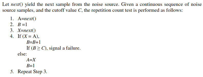
With the following criteria for failure:

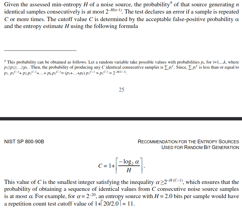
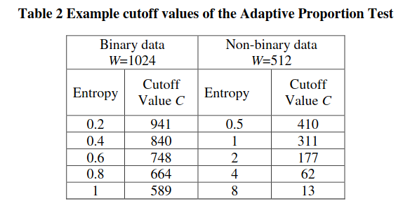
And this is the adaptive proportion test:

With the following example cutoff values:

OK, so now we know the tests. What do these even mean in the context of our TRNGs?

Ring Oscillator Implementations

Our Ring Oscillator architecture consists of 33 independent ring
oscillators that operate in two phases. In the first phase, the rings oscillate independently of each other to collect phase noise; the state of each ring is XOR’d into a state bit through snapshots taken at regular intervals. In a second phase, they are merged into a single large ring oscillator, where they then have to reach a consensus. A single bit is taken from the consensus oscillator, and progressively shifted into the state of the ring oscillator.

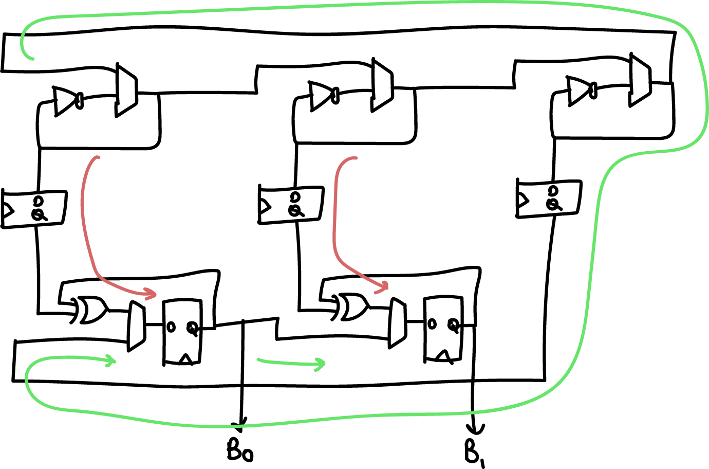
Above is a simplified “two bit” version of the generator, where instead of 33 oscillators we have 3, and instead of 32 bits of entropy we get 2. The red arrow is the flow of entropy in the first phase, and the green arrow is the flow of entropy in the second phase. The two phases are repeated N+1 bit times (33 times in the full implementation, 3 times in the simplified diagram above).

We can see from the diagram that entropy comes from the following
sources:

• Random phase accumulated in the smaller ring oscillators due to the accumulation of phase noise during a “dwell” phase that can be set by software (nominally 1000 ns)
• Decision noise associated with the sampling jitter of the smaller ring oscillators with an initial sampling flip-flop. Note that the ring oscillators operate at a higher frequency (~300-500MHz) than the sampling rate of the flip flops (100 MHz).
• Global phase accumulated during the consensus process of the larger ring oscillator. The time to achieve consensus is set by a “delay” parameter that is set by software (nominally 40ns)
• Cross-element mixing through the continuous shifting of bits to the right, and further XOR’ing of phase

The global phase consensus and cross-element mixing is quite important because ring oscillators have a tendency to couple and phase-lock due to crosstalk side-channels on both signal and power. In this architecture, each ring’s local noise conditions, including its crosstalk, is applied across each of the 32 output bits; and each ring’s oscillation is “reset” with an arbitrary starting value between each cross-element phase.

A higher rate of aggregate entropy is achieved by running four instances of the core described above in parallel, and XOR’ing their result together. In addition, the actual delay/dwell parameters are dynamically adjusted at run-time by picking some of the generated entropy and adding it to the base dwell/delay parameters.

Thus, when looking at this architecture and comparing it against the NIST spec, the question is, how do we apply the Repetition Count test and the Adaptive Proportion tests? The Repetition Count test is probably not sensitive enough to apply on the 32-bit aggregate output. It’s probably best to apply the Repetition Count and Adaptive Proportion test a bit upstream of the final generated number, at the sampled output of the ring oscillators, just to confirm that no constituent ring oscillator is “stuck” for any reason. However, the amount of logic resources consumed by adding this must be considered, since we have (33 * 4) = 132 separate oscillators to consider. Thus, for practical reasons, it’s only feasible to instrument one output from each of the four cores that is indicative of the health of the entire bank of oscillators.

Picking the right spot to instrument is tricky. The “large” ring oscillator is actually low-quality entropy, because it has a period of about 30MHz but is oversampled at 100MHz. Thus the majority of the entropy is contributed from the repeated undersampling of the “small” rings. The final sampling point chosen is the output of the sampling register after it’s “soaked up” enough entropy from the combination of a small ring and a large ring to result in a useful measurement.

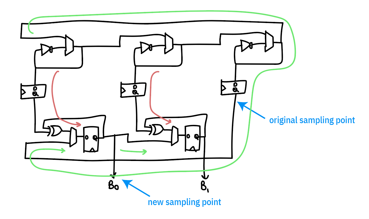
Originally, I had tried looking at the “large” oscillator only to try to find something more “raw”, under the hypothesis that we would be more likely to catch problems in the system at a less refined stage; the problem is that it was so “raw” that all we caught was problems. However, we do use this tap as a “true negative” test, to ensure that the health tests are capable of flagging an entropy source that is less than perfect.

I’m also going to introduce an extra test that’s inspired by the Runs Test in the STS suite, that I call “MiniRuns”. This test records the frequency of continuous runs of bits: 0/1, 00/11, 000/111, 0000/1111, etc. This test will offer more insight into the dominant projected failure mode of the ring oscillator, namely, it oscillating as a perfectly synchronized square wave — a condition that neither of the recommended NIST tests are capable of capturing. However, if the oscillator becomes too deterministic, we should see a shift in the distribution of run lengths out of the MiniRuns test.

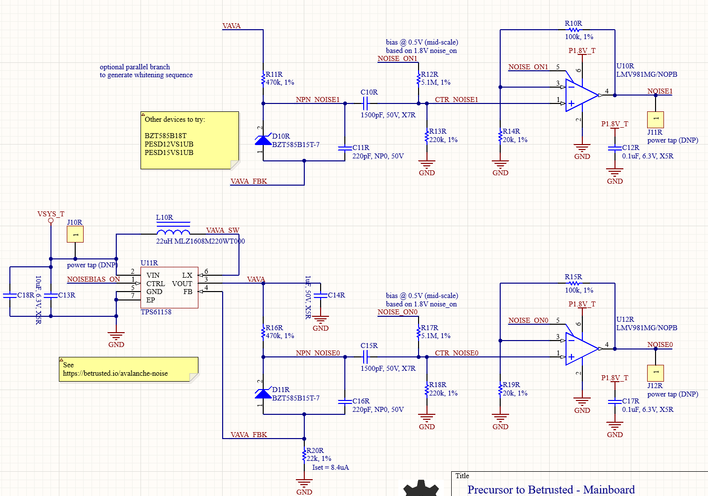
Avalanche Generator Implementation

The avalanche generator consists of two avalanche diodes biased from a shared power supply, sampled by a pair of op-amps with a slight bit of gain; see our page on its theory of
operation for details on the physics and electronic design. Here, we focus on its system integration. The outputs of each of the op-amps are sampled with a 12-bit ADC at a rate of ~1MSPS, and XOR’d together. As this sampling rate is close to the effective noise bandwidth of the diodes, we reduce the sampling rate by repeatedly shifting-by-5 and XOR’ing the results a number of times that can be set by software, nominally, 32 times into a 32-bit holding register, which forms the final entropy output. This 32x oversampling reduces the rate of the system to 31.25kHz.

Thus in this scheme, entropy comes from the following sources:

• The avalanche properties of two individual diodes. These are considered to be high-quality properties derived from the amplification of true thermal noise.
• The sampling interval of the ADC versus the avalanche waveform
• Noise inherent in the ADC itself
• Note that the two diodes do share a bias supply, so there is an opportunity for some cross-correlation from supply noise, but we have not seen this in practice.

Because we are oversampling the avalanche waveform and folding it onto itself, what we are typically measuring is the projected slope of the avalanche waveform plus the noise of the ADC. Significantly, the SNR of the Xilinx 7-series “12-bit” ADC integrated into our FPGA is 60dB. This means we actually have only 10 “good” bits, implying that the bottom two bits are typically too noisy to be used for signal measurements. The XADC primitive compensates for this noise by offering automatic averaging over 16 samples; we turn this off when sampling the avalanche noise generators, because we actually *want* this noise, but turn it on for all the other duties of the XADC.

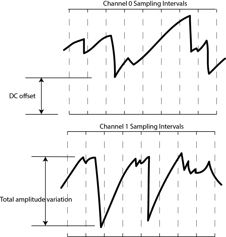
It’s also important to consider the nature of sampling this analog
waveform with an ADC. The actual waveform itself can have a DC offset, or some total amplitude variation, so naturally the LSBs will be dense in entropy, while the MSBs may be virtually constant. By focusing on the bottom 5 bits out of 12 with the 5-bit sliding window, we are effectively ignoring the top 7 bits. What does this do to the effective waveform? It’s a bit easier to show graphically:

Below is a waveform at full resolution.

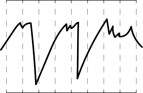
If we were to only consider 11 bits out of the 12, we effectively take half the graph and “wrap it over itself”, as shown below:

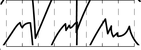
Down to 10 bits, it looks like this:

And down to 9 bits, like this:

And so forth. By the time we are down to just considering 5 bits, we’ve now taken the effective DC offset and amplitude variations and turned them into just another random variable that helps add to the entropy pool. Now take two of these, XOR them together, and add in the effective noise of the ADC itself, and you’ve arrived at the starting point for the ADC entropy pool.

In terms of on-line entropy tests, it probably makes the most sense to apply the Repetition Count test and the Adaptive Proportion tests to the bottom 5 bits of the raw ADC feed from each avalanche diode (as opposed to the full 12-bit output of the ADC). We don’t expect to hit “perfect entropy” with the raw ADC feed, but these tests should be able to at least isolate situations where e.g. the bias voltage goes too low and the avalanche effect ceases to work.

In addition to these tests, it’s probably good to have an “absolute
excursion” test, where the min/max of the raw avalanche waveforms are recorded over a time window, to detect a diode that is flat-lining due to aging effects, or a bias voltage source that is otherwise malfunctioning. This test is not suitable for catching if an attacker is maliciously injecting a deterministic waveform on top of the avalanche diodes, but is well-suited as a basic health check of the TRNG’s core mechanisms under nominal environmental conditions.

Developing

After installing the tooling necessary to build a Precursor/Betrusted SoC, I started writing the code.

Here’s the general method I use to develop code:

1. Think about what I’m trying to do. See the first section of this
   article.
2. Write the smaller submodules.
3. Wrap the smaller modules into a simulation framework that shakes
   most of the skeletons out of the closet.
4. Repeat 1-3, working your way up the chain until you arrive at your full solution.
5. Write drivers for your new feature
6. Slot your feature into the actual hardware
7. Test in real hardware
8. Continuously integrate, if possible, either by re-running your sim against every repo change or better yet recompiling and re-running your test on actual hardware.

The key to this loop is the simulation. The better your simulation, the better your outcome. By “better simulation”, I mean, the less
assumptions and approximations made in the test bench. For example, one could simulate a module by hooking it up to a hand-rolled set of Verilog vectors that exercises a couple read and write cycles and verifies nothing explodes; or, one could simulate a module by hooking it up to a fully simulated CPU, complete with power-on reset and multiple clock phases, and using a Rust-based framework to exercise the same reads and writes. The two test benches ostensibly achieve the same outcome, but the latter checks much more of the hairy corner cases.

For Betrusted/Precursor, we developed a comprehensive simulation framework that achieves the latter scenario as much as possible. We simulate a full, gate-level Vex CPU, running a Rust-built BIOS, employing as many of the Xilinx-provided hardware models as we can for things like the PLL and global power-on reset.

Demo

This is the point in the cooking show at which we put the turkey into an oven, say something to the effect of “…and in about five hours, your bird should be done…” yet somehow magically pull out a finished turkey for carving and presentation by the time we finish the sentence.

So: after a bunch more driver-writing and breaking out signals to gain visibility into the various metrics and failure modes, we can see the on-line health tests in action.

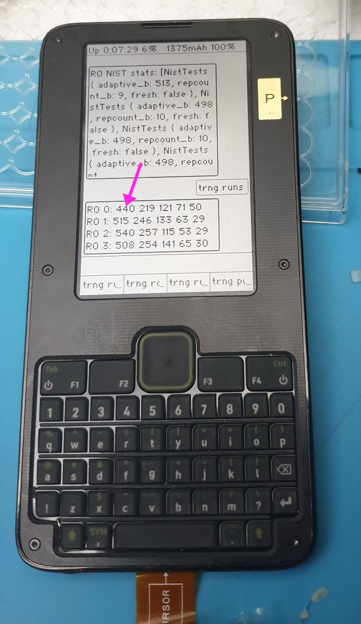
Above is an example of the trng test data output on Precursor, set where `RO 0` is connected to the “large” oscillator that runs too slowly (serving as a “true negative” test), and the others are connected to the final output tap for the test (serving as a “true positive”). In the output, you can see the four ring oscillators (numbered 0-3) with the frequency of each of five run lengths printed out. `RO 0` has a significant depression in the count for the run-length 1 bin, compared to the other oscillators (440 vs 515, 540, and 508).

One final detail is implementing an automated decision mechanism for the MiniRuns test. Since the MiniRuns test wasn’t from the NIST suite, I couldn’t simply read a manual to derive a threshold. Instead, I had to consult with my perlfriend, who also happens to be an expert at statistics, to help me understand what I was doing and derive a model that could help me set limits. Originally, she suggested a chi-square test. This would be great, but the math for it would be too complicated for an automated quick power-on test. So, we downgraded the test to simple max/min thresholds on the counts for each “bin” of runs. I used a similar criteria to that suggested in the NIST test, that is, alpha = 2^-20, to set the thresholds, and baked that into the hardware code. Here’s a link to the original spreadsheet that she used to compute both the chi-square and the final, simpler min/max tests. One future upgrade could be to implement some recurring process in Xous that collects updated results from the MiniRuns test and does the more sophisticated chi-square tests on it; but that’s definitely a “one for the road” feature.

Closing Thoughts
The upshot is that we now have all the mandatory NIST tests plus one each “tailored” tests for each type of TRNG. Adding the MiniRuns automated criteria increased utilization to 56.5% — raising the total space used by the tests from about 2% of the FPGA to a bit over 4%. The MiniRuns test is expensive because it is currently configured to check for runs ranging from length 1 to 5 over 4 banks of ring oscillators — so that’s 5 * 4 * (registers/run ~30?) = ~600 registers just for the core logic, not counting the status readout or config inputs.

Later on, if I start running out of space, cutting back on some of the instrumentation or the depth of the runs measured might be a reasonable thing to do. I would suggest disposing of some of the less effective NIST tests entirely in favor of the home-grown tests, but in the end I may have to kick out the more effective supplemental tests. The reality is that it’s much easier to defend keeping inferior-but-spec-compliant tests in the system, rather than opting for superior tests at the expense of the specification tests.

That’s it for part 1. If you’re super-eager to read more, you can read the full wiki entry on data conditioning for the TRNG at the Precursor/Betrusted documentation wiki. Or, you can just wait until I get around to chopping the page down to size and repackaging it into a more bite-side blog entry.

It was pointed out that we’re missing a step-by-step guide on how to go from an idea, to hardware, to a fully implemented feature in Xous for Precursor. So, here it is.

Because Precursor uses an FPGA for its SoC, we can add new features to the hardware “on the fly”. In this case, we’re going to add some improvements to our basic managed TRNG block. To review, the existing TRNG consists of an avalanche noise source and a ring oscillator noise source as hardware-based sources of “true” entropy. Two generators are used for the following reasons:

• An external discrete generator is easy to check (just put an oscilloscope on the avalanche noise source), but harder to protect against physical access attacks
• An integrated, on-chip generator is harder to hack (more robust against a pair of tweezers executing a short-to-ground attack, or RF interference attacks), but harder to check (is the data from the TRNG, or merely a decoy CSPRNG implant?)
• All hardware mechanisms are fallible; having two sources improves robustness against transient drop-outs or aging failures

We’ve already done extensive, months-long characterization of both of the TRNG sources and found them to produce passable raw entropy. However, the system is still missing two features that are generally considered to be best practice:

1. Independent, on-line health monitors of the raw TRNG outputs. It’s important that the health monitoring happens before any conditioning or mixing of the raw data happens, and significantly, there is no one-size-fits-all health monitor for a TRNG: it’s advised (NIST SP 800-90B sec 4.4) to have tests that are tailored to the noise source.
2. Conditioning of the raw data. Despite best efforts to make TRNGs unbiased and flawless, they are really hard to get right. Furthermore, they are only capable of producing high-quality entropy at a limited data rate. Thus, most practical systems take a TRNG output and run it through a cryptographic stream cipher to generate a final datastream; this simultaneously protects against minor flaws in the TRNG while improving the availability of random numbers.

The following lengthy posts walk step-by-step through the thought process, implementation and debugging process of adding these features. Few people would even notice these features, and if everything is doing its job right (that is, the TRNG’s raw data is working correctly) is indistinguishable from the state before all this effort. However, we take TRNGs seriously here; so much rides on the quality of these random numbers that it’s probably worth the effort to harden them against failures, be they unintentional, malicious, or just design bugs.

I have to be honest, I spent a lot of time to check a box that few people care about, but I’ve come to realize that’s mainly what writing OS code and firmware is about. You can get more fame and dopamine from creating a cool UI theme with an afternoon of work. It’s also really hard to explain to everyday people what you’re doing exactly with all this time and effort; but without the underlying frameworks that make things durable and reliable, we all might as well be drawing chalk pictures on the side walk.

Without further ado, here are the two guides for adding features, there’s some repetition between the posts so they can be read independently.

• On-line health monitors
• Raw data conditioning

I’ll also take highlights from these wiki articles and repost them to the blog here, creating a “TL;DR” version that is also neatly delivered to the inboxes of my blog’s email subscribers.